Understanding the Transformer

This article explains the landmark paper Attention Is All You Need by Vaswani et al. (2017), which introduced the Transformer architecture that powers GPT, BERT, and nearly every modern language model.

Introduction

How do you teach a model to relate any two words in a sentence, no matter how far apart they sit? For years the answer was to walk the sentence left to right and hope the signal survived the trip. The Transformer threw that assumption out.

Earlier sequence models—for translation, language modeling, generation—were built on recurrent or convolutional networks, usually with an encoder, a decoder, and an attention link between them. The Transformer keeps the attention link and discards everything else: no recurrence, no convolution. The result is a model that trains faster, parallelizes cleanly, and reaches higher quality.

The rest of this article builds the architecture one constraint at a time: first why sequential models hurt, then attention as the fix, then the full encoder-decoder stack.

The Sequential Bottleneck

Before the Transformer, the dominant approach to sequence tasks—machine translation, language modeling, text generation—was the recurrent neural network (RNN), particularly LSTMs and GRUs.

RNNs process sequences one token at a time. To compute the hidden state at position $t$, you need the hidden state at position $t-1$:

Read it plainly: the state at position $t$ is a function of the previous state and the current token. Position $t$ cannot start until position $t-1$ finishes. This creates two fundamental problems:

Lack of Parallelization

Because each step depends on the previous step, you cannot parallelize computation within a single sequence. Training is inherently sequential in time. For long sequences, this becomes a severe bottleneck.

Long-Range Dependencies

Information from early tokens must survive many sequential steps to influence later processing. Gradients must flow backward through all those steps. In practice, this makes learning long-range dependencies difficult, even with gating mechanisms like LSTM.

The answer is the Transformer.

Attention as a Lookup

The core idea of attention is surprisingly simple: it’s a soft lookup into a set of values, where the lookup key determines how much weight to give each value.

Think of it like a database query:

• You have a query (what you’re looking for)
• You have a set of keys (labels for stored items)
• You have a set of values (the stored items themselves)

The attention mechanism compares your query to each key, computes a relevance score, and returns a weighted combination of the values.

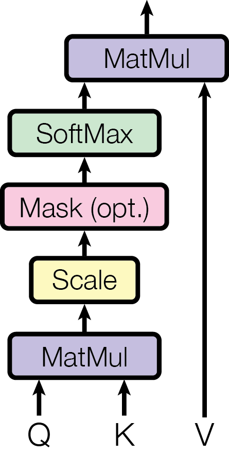
Scaled Dot-Product Attention

The Transformer uses a specific form of attention called Scaled Dot-Product Attention.

Given:

• Queries $Q \in \mathbb{R}^{n \times d_k}$ — what we’re looking for
• Keys $K \in \mathbb{R}^{m \times d_k}$ — what we’re looking in
• Values $V \in \mathbb{R}^{m \times d_v}$ — what we retrieve

The attention output is:

Step by step

1. Compute compatibility scores: $QK^T$ gives an $n \times m$ matrix of dot products. Entry $(i, j)$ measures how much query $i$ matches key $j$.

2. Scale: Divide by $\sqrt{d_k}$. Without scaling, large $d_k$ values push dot products into regions where softmax has very small gradients.

3. Normalize: Apply softmax row-wise. Each query now has a probability distribution over keys.

4. Retrieve: Multiply by $V$. Each output is a weighted combination of values.

Why scale?

For large $d_k$, the dot products $q \cdot k$ tend to have large magnitude (variance roughly $d_k$). This pushes softmax into saturated regions where gradients vanish. Scaling by $\sqrt{d_k}$ keeps the variance at 1.

A worked example with real numbers

Abstractions land cold, so let one query attend over three tokens with $d_k = 2$. The query is $q = [1,\ 0]$, and the three keys and values are:

The query matched “the” most strongly, so its value dominates the output—but every token still contributes. Attention is a soft blend, not a hard pick. Swap in a query that points toward “cat” and the second row would dominate instead. That is the entire mechanism; multi-head attention and the full stack just repeat it at scale.

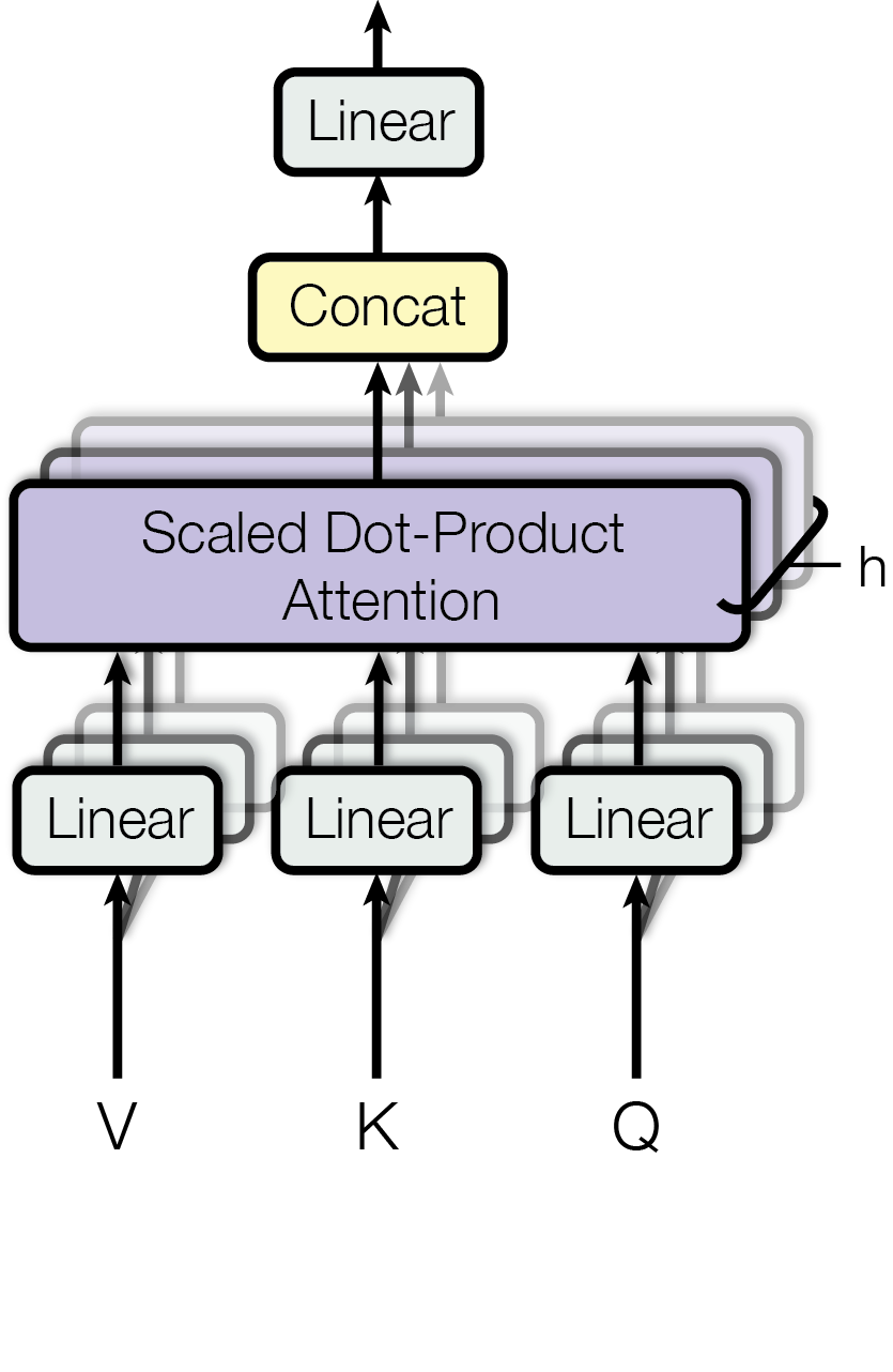
Multi-Head Attention

A single attention function can only focus on one type of relationship at a time. Multi-Head Attention runs multiple attention functions in parallel, each with its own learned projections.

Each head can learn to attend to different things:

• One head might focus on the previous word
• Another might focus on the subject of the sentence
• Another might focus on semantically similar words

The paper uses $h = 8$ heads with $d_k = d_v = 64$ (for $d_{\text{model}} = 512$). Each head works in a smaller 64-dimensional subspace, so eight heads cost about the same as one full-width head—the model gets several views of the sequence for the price of one.

The Transformer Architecture

The Transformer follows the encoder-decoder structure, but built entirely from attention and feed-forward layers.

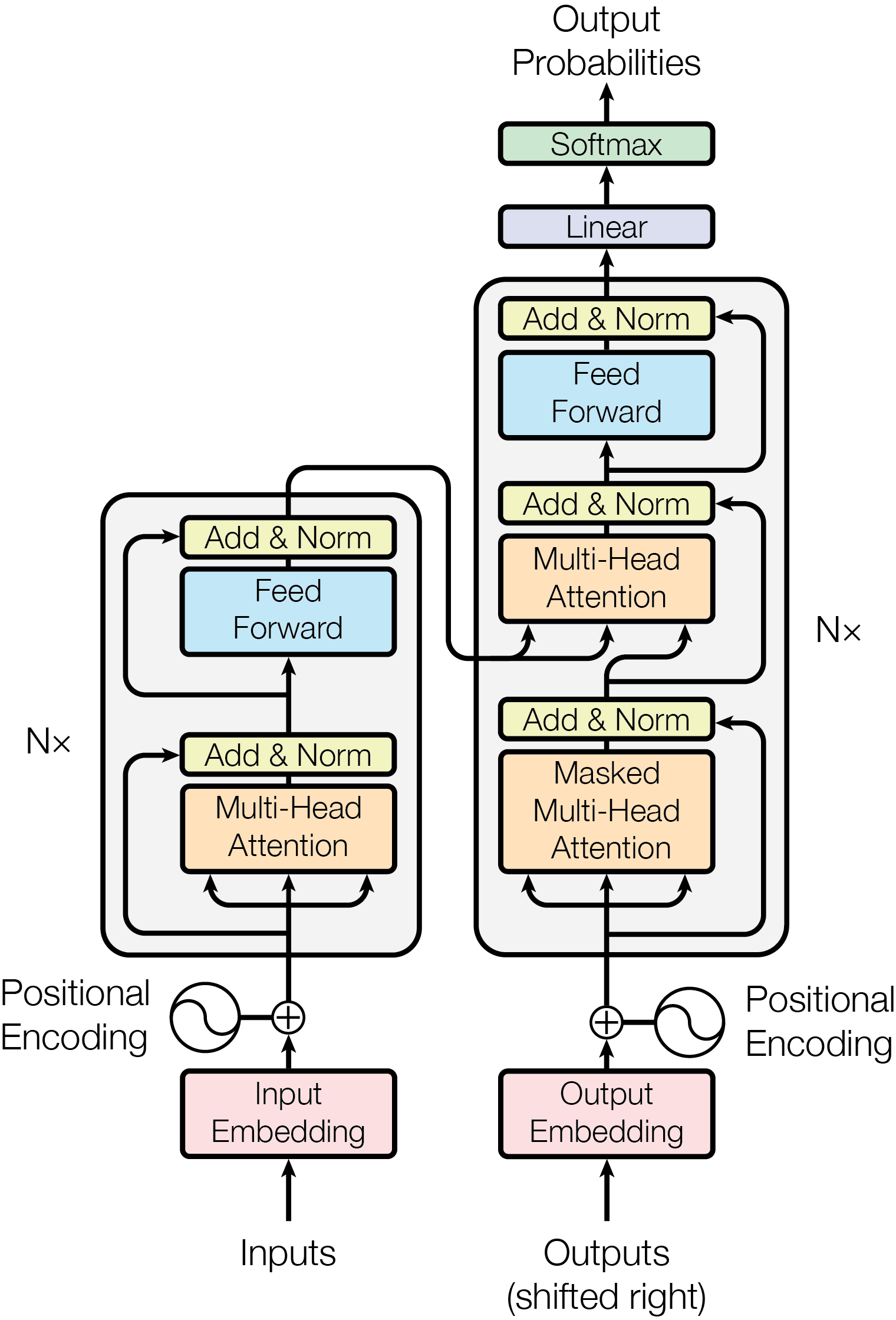
Encoder

Each encoder layer has two sub-layers:

1. Multi-head self-attention: Every position attends to every position
2. Feed-forward network: Applied independently to each position

In words: project each position up to a wider hidden size, apply a ReLU, project back down. Attention mixes information across positions; the feed-forward network then transforms each position on its own. The two sub-layers split the work: attention routes, the FFN thinks.

Residual connections and layer normalization wrap each sub-layer, which keeps gradients flowing through the deep stack.

Decoder

Each decoder layer has three sub-layers:

1. Masked self-attention: Each position attends only to earlier positions
2. Cross-attention: Queries from decoder; keys/values from encoder
3. Feed-forward network: Same as encoder

Positional Encoding

Attention treats its input as a set: shuffle the tokens and the output shuffles with them, unchanged. That is a problem—“dog bites man” and “man bites dog” would look identical. So before the first layer, the Transformer adds positional encodings to the input embeddings, giving each position a distinct fingerprint.

Each dimension $i$ is a sine or cosine wave of a different wavelength. Low dimensions oscillate slowly (they encode coarse position); high dimensions oscillate quickly (fine position). Together the waves form a unique code for every position—like the digits of a binary clock, but continuous.

For any fixed offset $k$, $PE_{pos+k}$ can be written as a linear function of $PE_{pos}$. This allows the model to learn to attend by relative position.

Why Self-Attention?

Self-attention connects all positions in $O(1)$ sequential operations, enabling full parallelization. It also provides a direct path between any two positions, making long-range dependencies easier to learn.

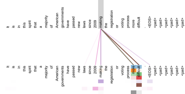
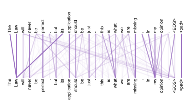
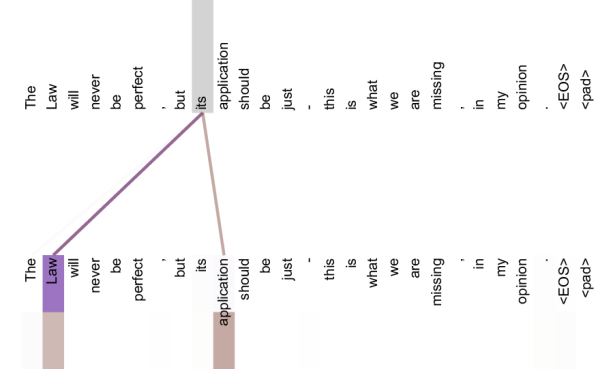
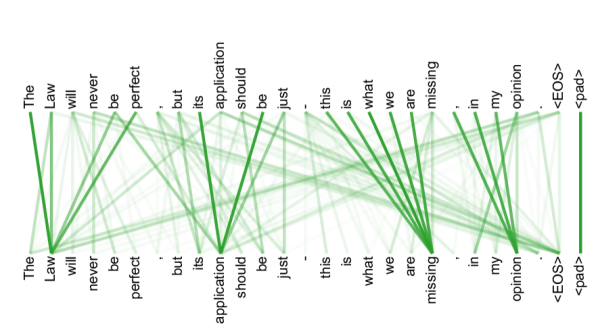
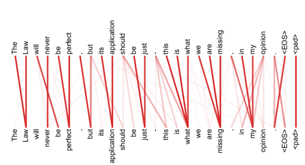
What Attention Heads Learn

The paper visualizes what individual attention heads learn in a trained Transformer. Different heads spontaneously specialize for different linguistic patterns—none of this structure is hard-coded.

Training and Results

Setup:

• Data: WMT 2014 English-German (4.5M pairs) and English-French (36M pairs)
• Hardware: 8 NVIDIA P100 GPUs
• Time: Base model 12 hours; Big model 3.5 days

The Transformer achieves state-of-the-art results at a fraction of the training cost.

The Lineage: One Block, Three Descendants

The paper shipped a full encoder-decoder for translation. What followed took the stack apart. The single self-attention block turned out to be reusable on its own, and the field split along the seam between encoder and decoder.

The masking rule is the whole difference. Remove the causal mask and every position sees the full sentence—that is BERT, tuned for understanding. Keep the mask so each position sees only its past, and you can generate one token at a time—that is GPT. Same block, one flag flipped.