 Michael Wan Interactive Insights
 This article explains mHC: Manifold-Constrained Hyper-Connections by Zhenda Xie, Yixuan Wei, Huanqi Cao et al. at DeepSeek (arXiv:2512.24880, December 2024). It traces a path from the residual connection (2015) through the layer normalization debate to ByteDance's Hyperconnections, then shows how DeepSeek uses convex geometry to make those connections trainable at scale.
Introduction
In January 2025, DeepSeek R1 briefly topped the App Store, beating ChatGPT and Gemini — trained at a fraction of the cost. When DeepSeek published mHC a month later, the question on everyone’s mind was whether this was the same kind of moment.
It isn’t a model release. It’s something quieter and, arguably, more interesting: a principled architectural improvement to how information flows between layers in a deep network. The key insight is geometric — the weight matrix governing that flow should live on the Birkhoff polytope, a beautiful object from combinatorics that ensures routing is always balanced.
To understand why that matters, we need to start at the beginning.
The Scaling Problem
The most natural way to make a neural network smarter is to make it deeper. More layers mean more computation, more abstraction, more capacity. But there’s a catch that plagued the field for years: simply stacking more layers often makes the model worse.
The culprit is the backpropagation chain rule. When you train a network, gradient signals flow backward from the loss through each layer. At every layer, the gradient is multiplied by that layer’s local Jacobian. For a network with $L$ layers:
$$\frac{\partial \mathcal{L}}{\partial h_0} = \prod_{l=1}^{L} \frac{\partial h_l}{\partial h_{l-1}}$$
This product of $L$ terms is the problem. If each term is slightly less than 1 — say, 0.9 — then after 50 layers the gradient is $0.9^{50} \approx 0.005$. After 100 layers: essentially zero. Gradients vanish, and early layers stop learning. Conversely, if each term is slightly greater than 1, gradients explode.

ResNet’s Answer — The Skip Connection
In 2015, He et al. solved this with a disarmingly simple idea: instead of hoping the gradient survives the entire chain, give it a shortcut. Add the input directly back to the transformed output.

The gradient of the loss with respect to $h_{l-1}$ now has two terms: one through $F$ (which may vanish) and one that is simply 1 (the identity path). No matter how deep the network, the gradient never has to multiply through a long chain alone. This single change won the 2015 ImageNet competition and became the standard building block for nearly every deep network since.
Where to Put Layer Norm
When the Transformer arrived in 2017, residual connections came along, but a new question emerged: where should you put Layer Normalization relative to the residual addition?

The original Transformer placed LayerNorm after the residual addition (Post-LN). This made gradients near the input unstable, requiring careful learning rate warmup and limiting how deep you could go.
GPT-2 moved LayerNorm before the sublayer (Pre-LN). Training became far more stable. But a new problem surfaced: in very deep Pre-LN networks, the residual stream accumulates scale. Each layer adds to it, and the pure residual path eventually dominates. Later layers contribute marginally — their outputs are tiny relative to the running sum. The representations in different layers start looking nearly identical. This is representation collapse.
Hyperconnections
In late 2024, researchers at ByteDance proposed a different approach. Instead of asking where to put LayerNorm within a fixed residual structure, they asked: what if you rethought the residual structure itself?
Their idea, called Hyperconnections (HC), replaces the single residual stream with $n$ parallel sub-streams. Each stream can receive contributions from all other streams, gated by a learned $n \times n$ weight matrix $W$:
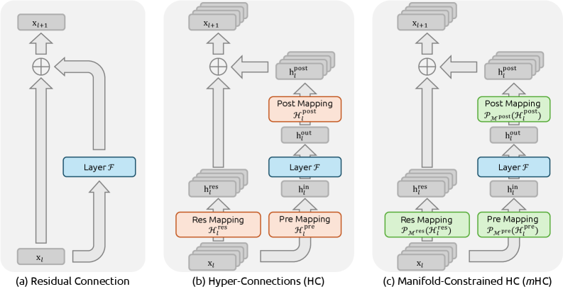
The update for stream $i$ at layer $l$ is:
This allows different parts of the representation to specialize independently — bypassing the seesaw between Post-LN and Pre-LN. The idea works.
But there’s a fatal flaw.
The Birkhoff Polytope
DeepSeek’s mHC keeps everything that makes Hyperconnections powerful, but adds one constraint: $W$ must be a doubly stochastic matrix.
Doubly Stochastic Matrices
A matrix $W \in \mathbb{R}^{n \times n}$ is doubly stochastic if all entries are non-negative and every row and every column sums to exactly 1:
Here’s a concrete $3 \times 3$ example:
| out 1 | out 2 | out 3 | Σ row | |
|---|---|---|---|---|
| in 1 | 0.75 | 0.14 | 0.11 | 1.00 |
| in 2 | 0.10 | 0.72 | 0.18 | 1.00 |
| in 3 | 0.15 | 0.14 | 0.71 | 1.00 |
| Σ col | 1.00 | 1.00 | 1.00 | — |
Intuitively, a doubly stochastic matrix is a conservative router: no stream receives more total weight than it sends, and vice versa. Information is redistributed, not amplified.
The Birkhoff Polytope
The set of all doubly stochastic matrices forms a convex polytope, called the Birkhoff polytope $\mathcal{B}_n$. Its vertices are exactly the $n!$ permutation matrices — the “pure routes” where each stream maps one-to-one to exactly one other stream. Everything inside is a convex mixture of these pure routes.

Why This Stabilizes Training
The key property is the spectral norm. For any $W \in \mathcal{B}_n$, its spectral norm (largest singular value) satisfies:
$$|W|_2 \leq 1$$
This follows from the Perron-Frobenius theorem: doubly stochastic matrices have leading eigenvalue exactly 1, and no eigenvalue exceeds 1 in magnitude. When you multiply by $W$ at every layer, the signal cannot grow. The 3,000× amplitude spike that broke vanilla Hyperconnections cannot happen inside $\mathcal{B}_n$.
The contrast in practice is striking. Figure 8 from the paper shows the actual learned weight matrices at individual layers and their cumulative product across 60 layers:

The Sinkhorn-Knopp Algorithm
The constraint $W \in \mathcal{B}_n$ is elegant, but how do you enforce it during gradient descent? You can’t simply clamp entries — that breaks the row and column sums simultaneously.
The answer is the Sinkhorn-Knopp algorithm (1967). After each gradient step updates $W$, you project it back onto the Birkhoff polytope by alternating two normalizations:
Each step is a single element-wise division. The algorithm converges to the unique doubly stochastic matrix closest to the input in KL divergence. In practice, 3–10 alternations suffice to reduce the maximum row/column deviation from 1 to below $10^{-3}$.
Interactive: Sinkhorn-Knopp Visualizer
Edit any cell in the matrix below, then step through the algorithm to watch it converge. Row sums and column sums turn green when they reach 1.
Sinkhorn-Knopp in Action
Start with any non-negative matrix. Each step alternates between row-normalizing and column-normalizing. Watch the sums (shown beside each row and column) converge to 1.
The mHC Formula
Putting it all together, the mHC forward pass is:
The difference from vanilla Hyperconnections is exactly one word: $W \in \mathcal{B}_n$. The forward computation is identical. The only extra work is running Sinkhorn-Knopp after each gradient step — a handful of element-wise divisions on an $n \times n$ matrix, negligible compared to the FFN or attention compute.
Training Dynamics and Results
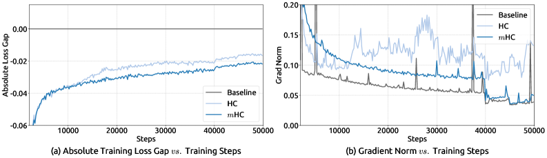
DeepSeek evaluated mHC at 3B, 9B, and 27B parameter scales using a MoE architecture based on DeepSeek-V3, with expansion rate $n = 4$ and Sinkhorn-Knopp iterations capped at $t_\text{max} = 20$.
Training stability (27B model). Figure 5 from the paper shows loss gap and gradient norm over 50K training steps:
Benchmark results (27B model, same token budget):
| Benchmark | Baseline | HC | mHC |
|---|---|---|---|
| BBH (EM) | 43.8 | 48.9 | 51.0 |
| DROP (F1) | 47.0 | 51.6 | 53.9 |
| GSM8K (EM) | 46.7 | 53.2 | 53.8 |
| HellaSwag (Acc.) | 73.7 | 74.3 | 74.7 |
| MATH (EM) | 22.0 | 26.4 | 26.0 |
| MMLU (Acc.) | 59.0 | 63.0 | 63.4 |
| PIQA (Acc.) | 78.5 | 79.9 | 80.5 |
| TriviaQA (EM) | 54.3 | 56.3 | 57.6 |
Key Takeaways
1. Depth needs highways. Residual connections are not an optional convenience — they’re what makes deep networks trainable. Without a bypass path, gradients vanish and early layers stop learning.
2. Hyperconnections generalize the residual. Three learned mappings (Res, Pre, Post) around each layer allow $n$ parallel streams to mix information flexibly, escaping the Post-LN / Pre-LN tradeoff. The idea is sound.
3. The Birkhoff polytope is the right constraint. Doubly stochastic matrices conserve signal magnitude ($|W|_2 \leq 1$) by construction. This turns a beautiful object from combinatorics into a practical stability guarantee for deep learning.
4. Sinkhorn-Knopp is the projector. Two alternating normalizations — row then column — converge to the unique doubly stochastic matrix nearest to the unconstrained gradient update. The compute cost is negligible.
5. mHC is a drop-in improvement. The only change relative to a standard Pre-LN Transformer is replacing the single residual stream with $n$ mHC streams and projecting $W$ after each optimizer step. Architecture, training recipe, and inference code are otherwise identical.
References
- Zhenda Xie et al. mHC: Manifold-Constrained Hyper-Connections. DeepSeek, 2024.
- Kaiming He et al. Deep Residual Learning for Image Recognition. CVPR 2016.
- Ashish Vaswani et al. Attention Is All You Need. NeurIPS 2017.
- Ruibin Xiong et al. On Layer Normalization in the Transformer Architecture. ICML 2020.
- Dingkang Sun et al. Hyper-Connections. arXiv 2024. (ByteDance)
- Richard Sinkhorn & Paul Knopp. Concerning nonnegative matrices and doubly stochastic matrices. Pacific Journal of Mathematics, 1967.
- Garrett Birkhoff. Tres observaciones sobre el álgebra lineal. Universidad Nacional de Tucumán, 1946.